Visualising Data with Improved Conditional Formatting

Conditional Formatting in Excel 2013 has been improved to let you quickly visualise and comprehend data. You’re going to find more styles, icons and data bars as well as the ability to highlight specified items like minimum and maximum values in just a few clicks.

• First of all highlight the data you want to apply the conditional formatting to.
• Go to the Home
  tab and in the Styles
  group select the Conditional
  Formatting
  button.

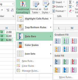
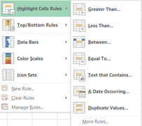
Some items in the drop down menu you may be familiar with already like Highlighting Cell Rules, Top/Bottom Rules, as these are the types of conditional formatting used in Excel 2003.

Data Bars, Colour Scales and Icon sets, calculate the format based on a comparison of the highlighted data.

You can modify the rules used from More Rules at the end of each list